German Tank Problem

Here we will cover a classic problem in statistics, estimating the total number of tanks from a small sample. Suppose four tanks are captured with the serial numbers 10, 256, 202, and 97. Assuming that each tank is numbered in sequence as they are built, how many tanks are there in total?

Since we are Bayesianists, we don’t want a singular estimate, we want a probability distribution for the total number of tanks. Therefore, we need to calculate the distribution of total tanks \(N\), given the serial numbers \(D\):

\[P(N \mid D) \propto P(D \mid N) \, P(N)\]

To build the model, first let’s think about the likelihood, \(P(D \mid N)\). For those not familiar with statistical notation, this is the probability that we would see these serial numbers, given the total number of tanks. To decide how to model the likelihood, we can think about how we would create our data. Simply, we just have some number of tanks, with serial numbers \(1, 2, 3, ..., N\), and we uniformly draw four tanks from the group. Therefore, we should use a discrete uniform distribution.

Next, we want to consider our prior information about \(N\), \(P(N)\). We know that it has to be at least equal to the largest serial number, \(m\). As for an upper bound, we can guess that it isn’t into the millions, since every serial number we saw is less than 300. We also know that \(N\) must be an integer and any value above 256 is equally likely, a priori, that is, before we saw the serial numbers. So a good choice here is the discrete uniform distribution again. I’ll set an upper bound at 10000, just to have it high enough for it not to affect our results. In statistical notation, we would write

\[\begin{split}P(N \mid D) &\propto P(D \mid N) \, P(N) \\ P(D \mid N) &\sim \mathrm{DiscreteUniform}(D, min=0, max=N) \\ P(N) &\sim \mathrm{DiscreteUniform}(N, min=m, max=10000) \\\end{split}\]

Now we can build the model with Sampyl and sample from the posterior.

import sampyl as smp
from sampyl import np

# Data
serials = np.array([10, 256, 202, 97])
m = np.max(serials)

# log P(N | D)
def logp(N):
    # Samplers will pass in floats, we need to make them integers
    N = np.floor(N).astype(int)

    # Log-likelihood
    llh = smp.discrete_uniform(serials, lower=1, upper=N)

    prior = smp.discrete_uniform(N, lower=m, upper=10000)

    return llh + prior

# Slice sampler for drawing from the posterior
sampler = smp.Slice(logp, {'N':300})
chain = sampler.sample(20000, burn=4000, thin=4)

posterior = np.floor(chain.N)
plt.hist(posterior, range=(0, 1000), bins=100,
         histtype='stepfilled', normed=True)
plt.xlabel("Total number of tanks")
plt.ylabel("Posterior probability mass")

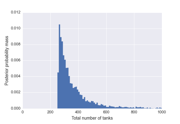
Above I’ve plotted the posterior distribution of \(N\). We can see that most of the probability is concentrated near the largest serial number in our data. In fact, the first 50% of the distribution is {256, 321}, and the first 95% is {256, 717}. This means there is a 50% probability that \(N\) lies below 321, and 95% probability it is below 717. As far as an estimate, I think these intervals are much more meaningful than the mean since the posterior is so skewed. However, I’ll report some of those statistics. The mean, median, and mode are 381.6, 321.0, 269, respectively.